Numerically Solving Planar Car Model with Pacejka Tire Model and Load Transfer

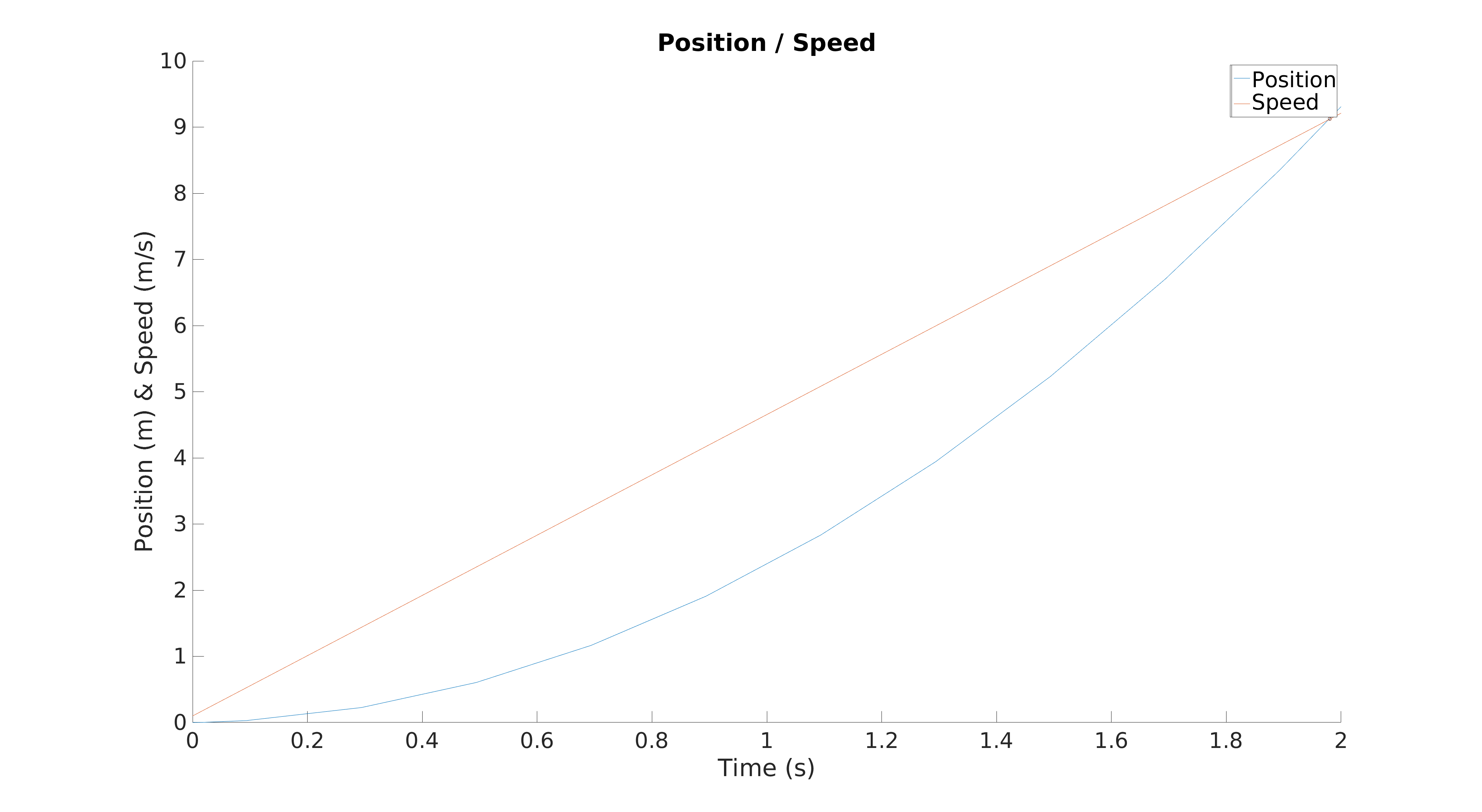
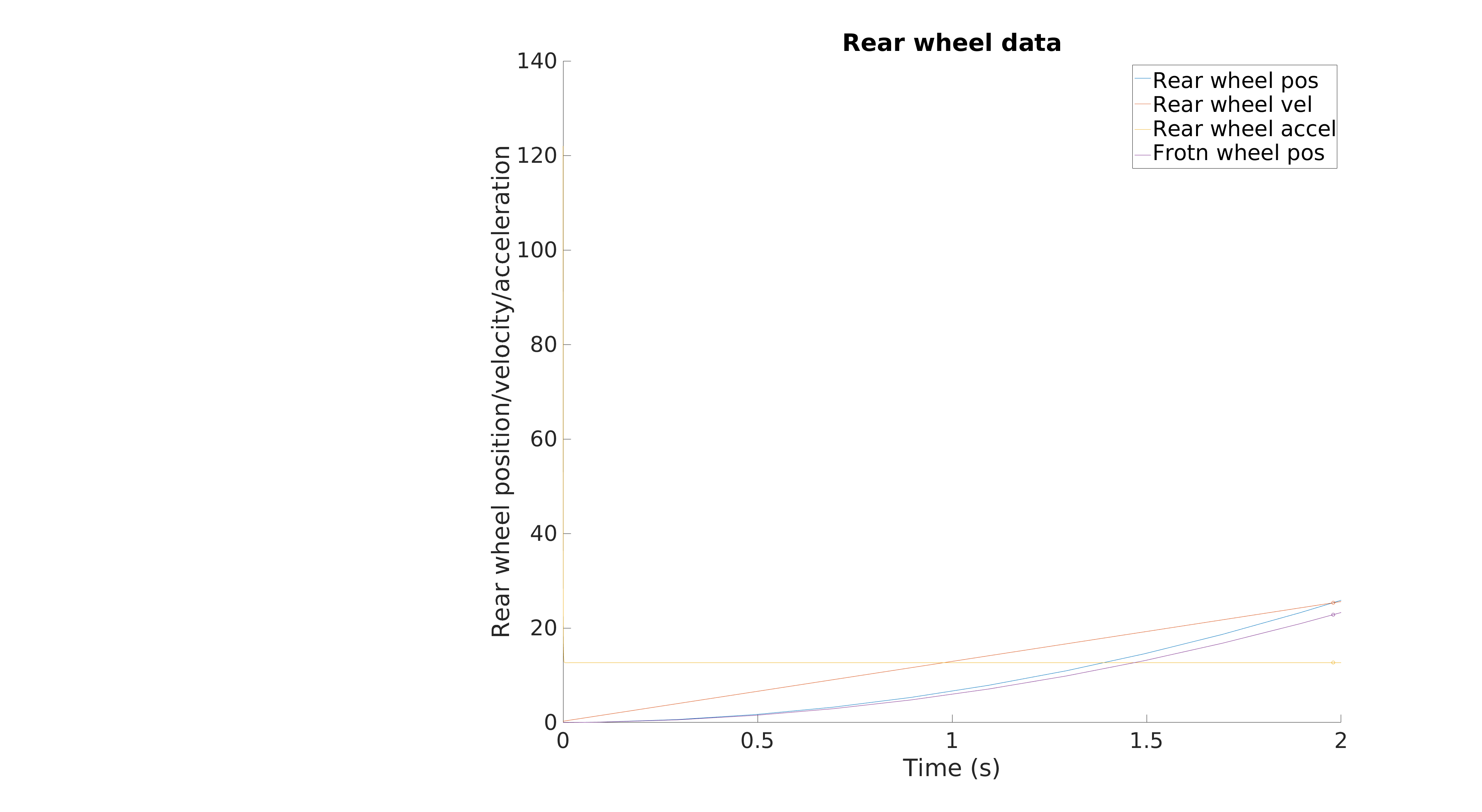
Consider a planar, rear-wheel-drive car viewed from the side. The state $$y$$ of the car is given by $$x, \dot{x}, \phi _{rear}, \dot{\phi} _{rear}$$, where $$x$$ and $$\dot{x}$$ represent the position and velocity of the car while $$\phi _{rear}$$ and $$\dot{\phi} _{rear}$$ represent the angular position and angular velocity of the rear wheel of the car. The front wheel of the car is assumed to be rolling with no slip and therefore doesn’t need any additional state variable.

Dynamics

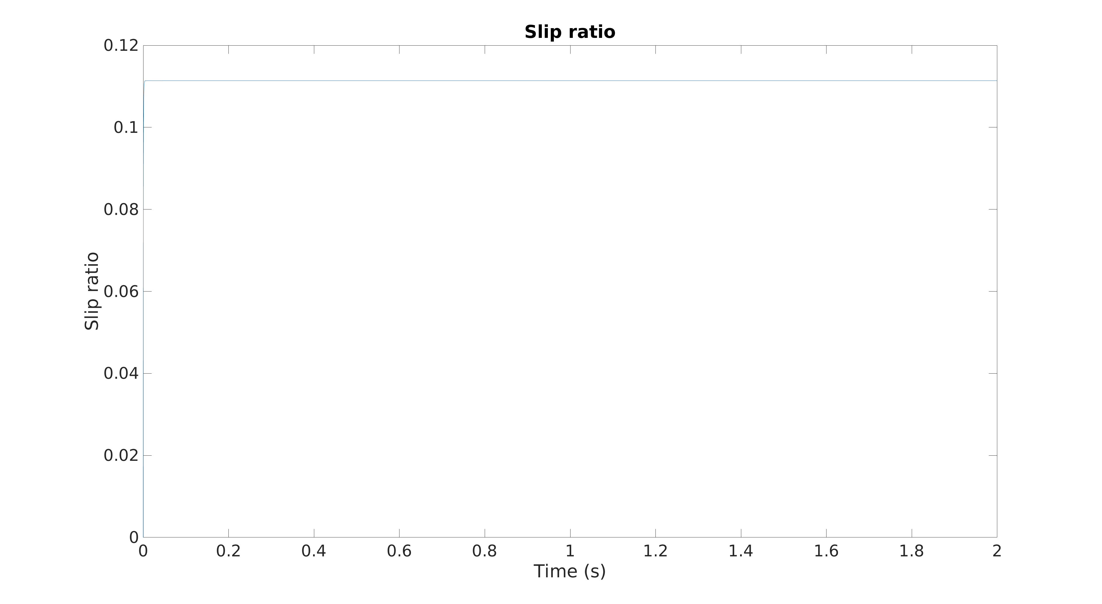
The slip ratio of the rear tire is defined as:

\begin{equation}
SR = \frac{\dot{\phi} _{rear} \cdot r}{\dot{x}} – 1
\end{equation}

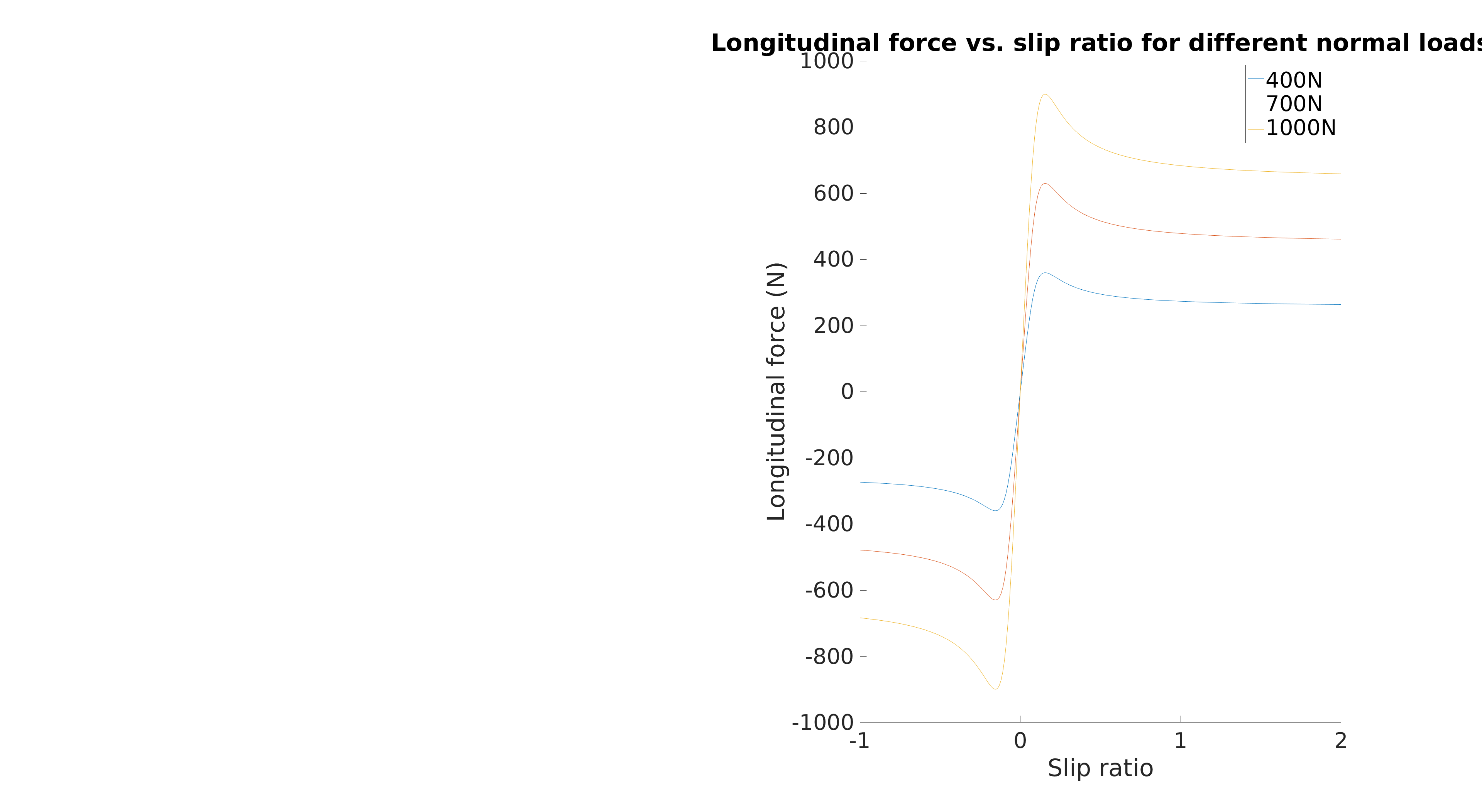
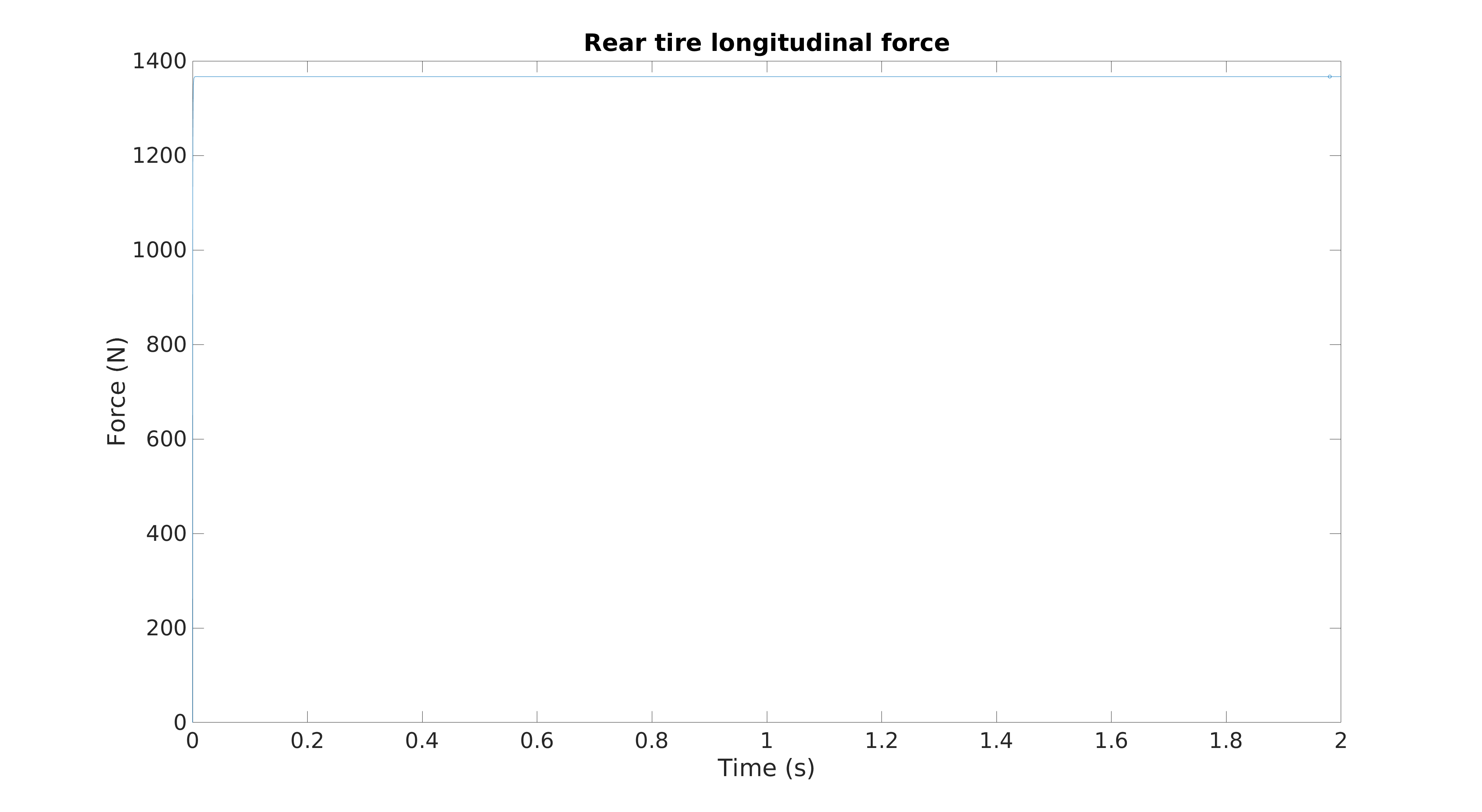
Where $$r$$ is the radius of the tire. Intuitively, this means that a slip ratio of -1 corresponds to a locked tire (full brakes), 0 corresponds to a free-rolling tire without slip, and positive numbers correspond to a tire that is spinning out against the pavement. The longitudinal force (forwards/backwards) is a function of the slip ratio and the vertical load on the tire. This relationship is empirically determined via the Pacejka Magic Tire Model, which results in graphs resembling the following:

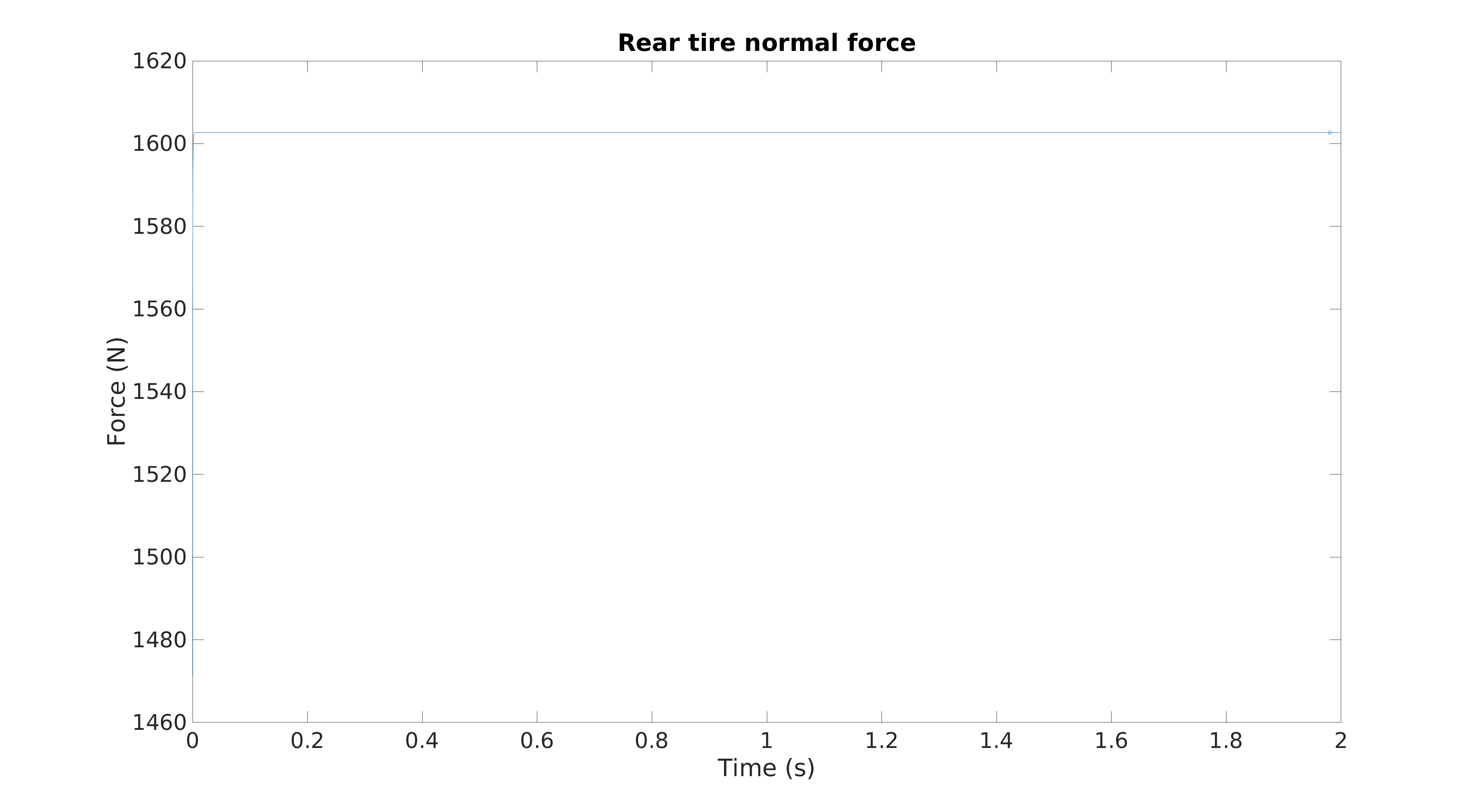
When deriving the car dynamics, weight transfer due to the acceleration of the car also needs to be considered. This is given by the following equation:

\begin{equation}
F_{rz} = \frac{mg}{2} + \frac{F_{rx} h}{l}
\end{equation}

Where $$m$$ is the mass of the car, $$g$$ is the gravitational constant, $$h$$ is the height of the COM of the car above the center of the wheels, $$l$$ is the wheelbase of the car, and $$F_{rz}$$ and $$F_{rx}$$ are the vertical and longitudinal forces on the rear tire, respectively. Recall that $$F_{rx}$$ is a function of $$F_{rz}$$ and $$SR$$.

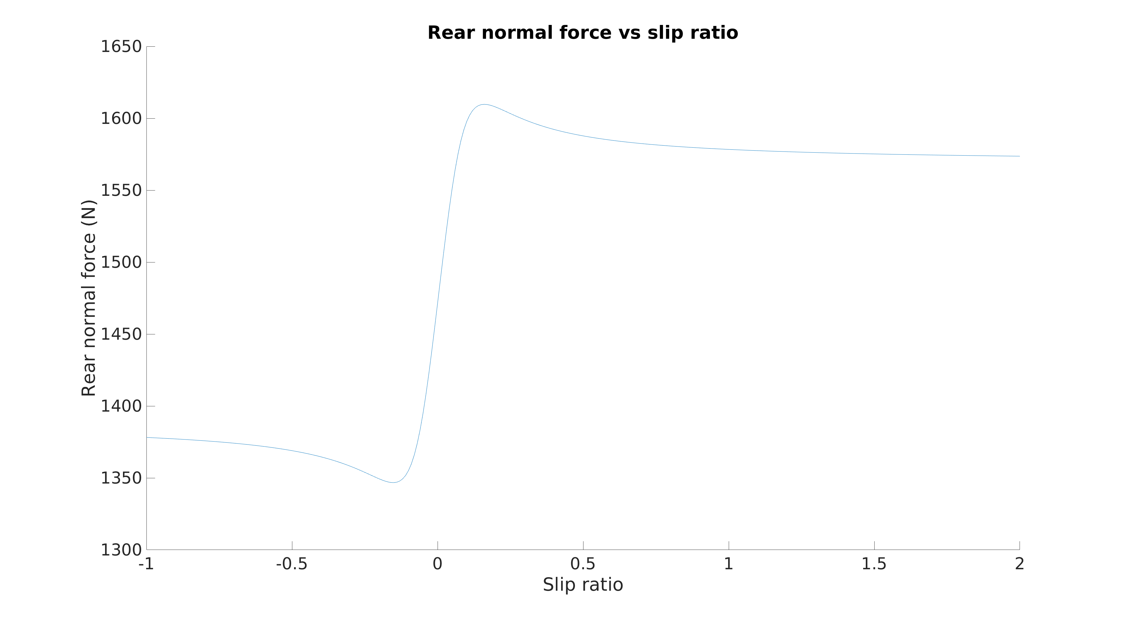
We want to ultimately know $$F_{rz}$$ as a function of only $$SR$$. The above equation isn’t analytically solvable for $$F_{rz}$$ since the black-box expression for $$F_{rx}$$ is rather complicated. To circumvent this, we numerically solve $$F_{rz}$$ for different values of $$SR$$ and fit the following curve (note the similarities with the Pacejka tire model):

We now can compute the derivatives of the state variables as follows:

\begin{equation}
\dot{y} = [y[2], F_{rx} / m, y[4], \frac{\tau – r \cdot F_rx}{I}]
\end{equation}

Where $$\tau$$ is the motor torque at the rear wheel and $$I$$ is the rotational inertia of the rear wheel.

Code

syms Frz SR

% Initialize car parameters
cp.halfLen = 1; % Wheel base divided by two
cp.height = 0.2; % COM height above center of wheels (halfway between wheels)
%cp.radius = 0.15; % Wheel radius
cp.radius = 0.4; % Wheel radius
cp.mass = 300; % Mass of car
cp.gravity = 9.8;
cp.wheelI = 5;
cp.vx0 = 0.1;
cp.MF52_par = [1.5 900 -0.256 -2 0 0 0 100 0 0 0 0 0 0];

%grid on
%}

% Get longitudinal force as a function of syms Frz and SR
Frx = MF52_LongForce_calc(cp.MF52_par, SR*100, Frz);
Frx = Frx{1};

% Dynamics equation
if ~isfield(cp, 'frzFit')
    % Equation relating Frz and SR; not directly solvable for Frz
    dynamicsEqn = Frz == cp.mass * cp.gravity / 2 + Frx * cp.height / (2 * cp.halfLen);
    dynamicsEqn = simplify(dynamicsEqn);
    % Numerically solve for Frz as a function of SR and approximate
    cp.frzFit = solveFrz(dynamicsEqn);
end

% [x, xdot, phiRear, phiRearDot]
% phiRear is not actually required, it's just for rendering purposes
stateI = [0, cp.vx0, 0, cp.vx0 / cp.radius];

% The system is stiff! We need a stiff solver
% What makes a system stiff?
[t, y] = ode23s(@(time, state) dynamics(time, state, cp), [0, 2], stateI.');

simOut.t = t;
simOut.cp = cp;
simOut.dynamicVars = unpackState(y);

% Copy all the dynamics debug output into simulation output
for i = 1:length(t)
    [~, debug] = dynamics(t(i), y(i, :)', cp);
    f = fieldnames(debug);
    for k = 1:length(f)
        simOut.dynamicVars.(f{k})(:, i) = debug.(f{k});
    end
end

function [dydt, debug] = dynamics(t, y, cp)
    state = unpackState(y);
    sr = state.prdot * cp.radius / state.xdot - 1;
    frz = feval(cp.frzFit, sr);
    frx = MF52_LongForce_calc(cp.MF52_par, sr*100, frz);
    frx = frx{1};
    %inputTorque = 20 * cos(t);
    inputTorque = 610; 
    netTorque = inputTorque - cp.radius * frx;
    
    dydt = [state.xdot; frx / cp.mass; state.prdot; netTorque / cp.wheelI];
    debug.frx = frx;
    debug.frz = frz;
    debug.sr = sr;
    debug.prddot = netTorque / cp.wheelI;
end

function [frzFit] = solveFrz(momentEqn)
    syms Frz SR

    SRs = -1:0.1:2;
    % Frzs contains the rear normal force over a range of slip ratios
    Frzs = arrayfun(@(slipRatio) double(vpasolve(subs(momentEqn, SR, slipRatio), Frz)), SRs);

    maxFrz = max(Frzs);
    minFrz = min(Frzs);
    % Will be the rough vertical positioning of the fitted Frz
    vShift = -maxFrz + (maxFrz - minFrz) / 2;

    startB = -7;
    startC = -1.5;
    startD = 500;
    startE = -4;
    startF = 0;
    startG = -vShift;
    
    % Numerically fit an approximation for the black-box function
    ft = fittype('d * sin(c * atan(b * (1-e) * (k+f) + e * atan(b * (k+f)))) + g', ...
        'dependent', 'Frx', 'independent', 'k', 'coefficients', {'b','c','d','e', 'f', 'g'});
    % Gives rear tire normal force as a function of slip ratio
    frzFit = fit(SRs.', Frzs.', ft, 'StartPoint', [startB, startC, startD, startE, startF, startG]);

    %plot(frzFit, SRs, Frzs);
    % model = @(k) startD * sin(startC * atan(startB * (1-startE) * (k-startF) + startE * atan(startB * (k-startF)))) + startG;
    %plot(SRs, arrayfun(model, SRs));
end