Numerically Solving Discrete Systems with Mathematica for Robocode

As a learning project, I’ve been trying to forwards-integrate Robocode physics using Mathematica. Robocode is a programming game where two or more tanks battle in a 2D arena, attempting to hit enemies while simultaneously dodging bullets. In order to better determine all the possible locations my tank could move to given an initial state and fixed time horizon, I decided to use Mathematica to numerically integrate Robocode tank physics over a range of different control inputs. Ultimately, I was quite impressed with how Mathematica’s NDSolve could handle some weird discrete physics—however, there are a lot of tricky issues that you have to watch out for (hence why I’m writing this post).

Robocode Physics

Robocode works with discrete time steps called ticks. We’ll describe our tank’s state using four variables: the position , the velocity , and the orientation .

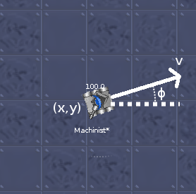
The movement physics are described here so I won’t go over them in detail. The control inputs are the acceleration , with a maximum of 1 when accelerating and 2 when decelerating, and the angular velocity , bounded by .

The integration scheme is essentially Implicit Euler with constant step sizes of one tick (however, this has some caveats as we’ll find later). There’s a lot of other weird corner cases that make this problem more difficult than it first appears. My hope is by going through and addressing these issues you can learn why your numerical solution for discrete systems is misbehaving. We’ll start with a simple, naive approach and build up from there.

Just Pretend it’s Continuous (Try #1)

Let’s first try to formulate the dynamics by ignoring the discrete time steps. For simplicity we’ll also ignore deceleration and assume the tank accelerates from rest in a straight line. This looks like the following:

tEnd = 10; (* Finish time of simulation *)

dynamics = {

(* Set velocity derivative to target acceleration *)

veqn = v'[t] == ta[t],

(* Set turn rate to target, but clamp between physical limits *)

ϕeqn = ϕ'[t] == Clip[tω[t], {-10 Degree + 3/4 Degree * v[t], 10 Degree – 3/4 Degree * v[t]}],

xeqn = x'[t] == v[t]*Cos[ϕ[t]],

yeqn = y'[t] == v[t]*Sin[ϕ[t]]

};
(* Add dynamics equations and initial conditions *)

soln = NDSolve[{dynamics, x[0]==0, y[0]==0, ϕ[0]==0 Degree,

v[0]==0, tω[0]==0 Degree, ta[0]==1,

(* When velocity reaches maximum, stop acceleration *)

WhenEvent[Evaluate[v[t] == 8], {ta[t]->0}]},

(* Specify desired outputs and integration timeframe *)

{x, y, x’, y’, v, ϕ, ϕ’}, {t, 0, tEnd},

(* Allow target turn / accelerate variables to jump discontinuously *)

DiscreteVariables->{tω, ta}];
(* Plot solution *)

ParametricPlot[Evaluate[{x[t], y[t]} /. soln], {t, 0, tEnd}]

(* Output end position *)

posEnd = Evaluate[{x[t], y[t]} /. soln] /. t->tEnd

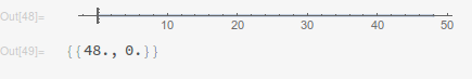
At first glance this seems reasonable; since we didn’t turn at all, the tank went straight to the right and ended up traveling 48 pixels in 10 ticks. Let’s compare this to actual measurements from Robocode for maximal acceleration from rest:

Tick #0
Displacement: [0.0, -0.0]
Velocity: [0.0, 0.0], abs: 0.0
Tick #1
Displacement: [0.9999999999999869, -1.73749903353837E-14]
Velocity: [1.0, 2.7755575615628914E-16], abs: 1.0
Tick #2
Displacement: [2.999999999999961, -5.218048215738236E-14]
Velocity: [2.0, 5.551115123125783E-16], abs: 2.0
Tick #3
Displacement: [5.999999999999984, -9.769962616701378E-15]
Velocity: [3.0, 6.661338147750939E-16], abs: 3.0
Tick #4
Displacement: [10.000000000000007, 7.105427357601002E-15]
Velocity: [4.0, 1.1102230246251565E-15], abs: 4.0
Tick #5
Displacement: [15.000000000000004, 1.509903313490213E-14]
Velocity: [5.0, 1.7763568394002505E-15], abs: 5.0
Tick #6
Displacement: [20.999999999999986, 5.329070518200751E-15]
Velocity: [6.0, 1.3322676295501878E-15], abs: 6.0
Tick #7
Displacement: [27.999999999999957, -2.1316282072803006E-14]
Velocity: [7.0, 1.3322676295501878E-15], abs: 7.0
Tick #8
Displacement: [35.99999999999998, 2.8421709430404007E-14]
Velocity: [8.0, 2.220446049250313E-15], abs: 8.0
Tick #9
Displacement: [44.0, 7.815970093361102E-14]
Velocity: [8.0, 2.220446049250313E-15], abs: 8.0
Tick #10
Displacement: [52.00000000000002, 1.3145040611561853E-13]
Velocity: [8.0, 2.220446049250313E-15], abs: 8.0

At tick 10, we see that the tank has actually traveled 52 pixels (ignoring rounding errors). What gives? The key lies in looking at the data for the first tick. After one tick, the Robocode tank has traveled 1 pixel and has a velocity of one pixel/tick. Our Mathematica solution after one tick gives the robot a velocity of one tick per second but only says it’s moved half a pixel. This discrepancy is due to the Robocode’s Implicit Euler integration scheme, where the change in position between two ticks is equal to the velocity at the later tick times the time difference.

Implicit Euler Integration (Try #2)

Let’s try making NDSolve use Implicit Euler with a fixed step size of one. The first thing to note is that while Mathematica supplies a built-in ExplicitEuler method, we have to supply our own Implicit Euler definition (taken from here). The step size is specified using the “StartingStepSize” argument. Our code then looks like the following:

tEnd = 10; (* Finish time of simulation *)

dynamics :=

{

veqn = v'[t] == ta[t],

(* Set turn rate to target, but clamp between physical limits *)

ϕeqn = ϕ'[t] == Clip[tω[t], {-10 Degree + 3/4 Degree * v[t], 10 Degree – 3/4 Degree * v[t]}],

xeqn = x'[t] == v[t]*Cos[ϕ[t]],

yeqn = y'[t] == v[t]*Sin[ϕ[t]]}
(* Implicit Euler is not implemented directly, must define ourselves *)

(* Robocode does Implicit Euler for physics *)

ImplicitEuler = {"FixedStep", Method -> {"ImplicitRungeKutta",

"Coefficients" -> "ImplicitRungeKuttaRadauIIACoefficients",

"DifferenceOrder" -> 1, "ImplicitSolver" -> {"FixedPoint",

AccuracyGoal -> MachinePrecision, PrecisionGoal -> MachinePrecision,

"IterationSafetyFactor" -> 1}}};
(* Add dynamics equations and initial conditions (starting velocity must be non-zero,

so I just add a negligible x'[0] to give a direction to move in *)

soln = NDSolve[{dynamics, x[0]==0, y[0]==0, ϕ[0]==0 Degree,

v[0]==0, tω[0]==0 Degree, ta[0]==1,

(* When velocity reaches maximum, stop acceleration *)

WhenEvent[Evaluate[v[t] == 8], {ta[t]->0}]},

(* Specify desired outputs and integration timeframe *)

{x, y, x’, y’, v, ϕ, ϕ’}, {t, 0, tEnd},

(* Allow target turn / accelerate variables to jump discontinuously *)

DiscreteVariables->{tω, ta},

(* Use a ImplicitEuler method with a step size of one tic (matches robocode) *)

StartingStepSize->1, Method->ImplicitEuler];
(* Plot solution *)

ParametricPlot[Evaluate[{x[t], y[t]} /. soln], {t, 0, tEnd}]

(* Output end position *)

posEnd = Evaluate[{x[t], y[t]} /. soln] /. t->tEnd

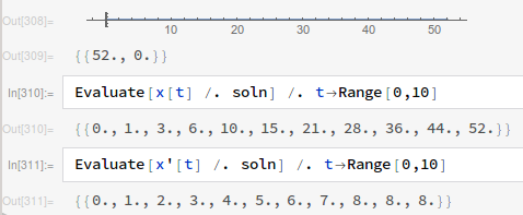
And we get the following output:

What? 48 again? I thought Implicit Euler integration was supposed to fix that. Closer inspection reveals that the WhenEvent might be the problem:

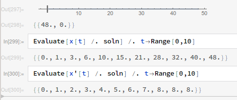
As you can see, the Implicit Euler integration matches the Robocode physics right up until the WhenEvent occurs at . This might actually be a bug in Mathematica since there’s no reason why the position should only change by four when the surrounding velocities are 7 and 8 pixels per tick. In fact, it seems like the WhenEvent is doing its job just fine (velocity goes up by one each tick and then stays at 8). After some frustrated debugging, I found that setting the WhenEvent’s LocationMethod to “StepEnd” like so:

WhenEvent[Evaluate[v[t] == 8], {ta[t]->0}, "LocationMethod"->"StepEnd" 

Fixes the issue.

Okay, good. It matches. I’m not quite sure why that worked, but I think there might be something funky going on with Mathematica under the hood. Let’s continue and add some turn in there (set ) and compare with Robocode:

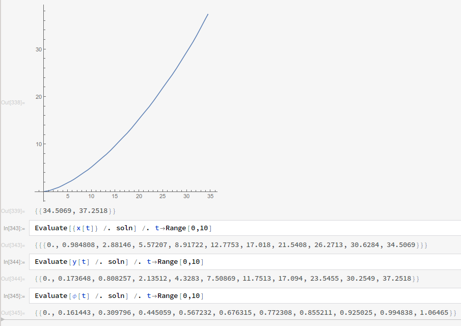
Tick #0
Displacement: [0.0, -0.0]
Velocity: [0.0, 0.0], abs: 0.0
Heading: 0.0
Tick #1
Displacement: [0.9848077530122417, 0.17364817766694823]
Velocity: [0.9848077530122081, 0.17364817766693], abs: 1.0
Heading: 0.17453292519943275
Tick #2
Displacement: [2.8729857937978536, 0.8330294681925363]
Velocity: [1.8881780407855688, 0.6593812905255734], abs: 2.0
Heading: 0.33597588100890796
Tick #3
Displacement: [5.52794870618697, 2.229873029167883]
Velocity: [2.654962912389127, 1.3968435609753318], abs: 3.0000000000000004
Heading: 0.4843288674284256
Tick #4
Displacement: [8.78441077961228, 4.552684852011626]
Velocity: [3.25646207342528, 2.3228118228437546], abs: 4.0
Heading: 0.6195918844579857
Tick #5
Displacement: [12.47079746366291, 7.930635890089924]
Velocity: [3.6863866840506243, 3.3779510380782978], abs: 5.000000000000001
Heading: 0.7417649320975892
Tick #6
Displacement: [16.42687235426334, 12.441674734963785]
Velocity: [3.9560748906004157, 4.511038844873862], abs: 5.999999999999999
Heading: 0.8508480103472351
Tick #7
Displacement: [20.516620013725372, 18.12269260871884]
Velocity: [4.089747659462047, 5.681017873755083], abs: 7.000000000000001
Heading: 0.946841119206923
Tick #8
Displacement: [24.636924613005846, 24.980031014335722]
Velocity: [4.120304599280439, 6.857338405616895], abs: 8.0
Heading: 1.0297442586766539
Tick #9
Displacement: [28.268848610922262, 32.10808320784266]
Velocity: [3.6319239979163793, 7.128052193506941], abs: 8.0
Heading: 1.0995574287564271
Tick #10
Displacement: [31.394697638836412, 39.47212203546218]
Velocity: [3.125849027914194, 7.364038827619521], abs: 8.0
Heading: 1.1693705988362004

The end position is way off, but more informative is the fact that after the first tick, the Robocode tank rotated by a full 10 degrees (0.1745 radians) whereas the Mathematica simulation rotated by just 9.25 degrees (0.1614 radians). The Mathematica result is to be expected since in the dynamics we clipped the rotational velocity to be and after one tick with maximum acceleration the velocity should equal one. However, the fact that the Robocode tank rotated a full ten degrees indicated that the rotational bounds were actually computed using velocity from the last tick; this was confirmed by looking at the Robocode source.

Delay Differential Equations (Try #3)

Let’s try using a delay differential equation to incorporate last tick’s translational velocity in the angular velocity bounds. Note the “v-1” in the dynamics equations:

tEnd = 10; (* Finish time of simulation *)

dynamics :=

{

veqn = v'[t] == ta[t],

(* Set turn rate to target, but clamp between physical limits *)

ϕeqn = ϕ'[t] == Clip[tω[t], {-10 Degree + 3/4 Degree * v[t-1], 10 Degree – 3/4 Degree * v[t-1]}],

xeqn = x'[t] == v[t]*Cos[ϕ[t]],

yeqn = y'[t] == v[t]*Sin[ϕ[t]]}
(* Implicit Euler is not implemented directly, must define ourselves *)

(* Robocode does Implicit Euler for physics *)

ImplicitEuler = {"FixedStep", Method -> {"ImplicitRungeKutta",

"Coefficients" -> "ImplicitRungeKuttaRadauIIACoefficients",

"DifferenceOrder" -> 1, "ImplicitSolver" -> {"FixedPoint",

AccuracyGoal -> MachinePrecision, PrecisionGoal -> MachinePrecision,

"IterationSafetyFactor" -> 1}}};
(* Add dynamics equations and initial conditions (starting velocity must be non-zero,

so I just add a negligible x'[0] to give a direction to move in *)

soln = NDSolve[{dynamics, x[0]==0, y[0]==0, ϕ[0]==0 Degree,

v[0]==0, tω[0]==10 Degree, ta[0]==1,

(* When velocity reaches maximum, stop acceleration *)

WhenEvent[Evaluate[v[t] == 8], {ta[t]->0}, "LocationMethod"->"StepEnd"]},

(* Specify desired outputs and integration timeframe *)

{x, y, x’, y’, v, ϕ, ϕ’}, {t, 0, tEnd},

(* Allow target turn / accelerate variables to jump discontinuously *)

DiscreteVariables->{tω, ta},

(* Use a ImplicitEuler method with a step size of one tic (matches robocode) *)

StartingStepSize->1, Method->ImplicitEuler];
(* Plot solution *)

ParametricPlot[Evaluate[{x[t], y[t]} /. soln], {t, 0, tEnd}]

(* Output end position *)

posEnd = Evaluate[{x[t], y[t]} /. soln] /. t->tEnd

Let’s have a look at our new output:

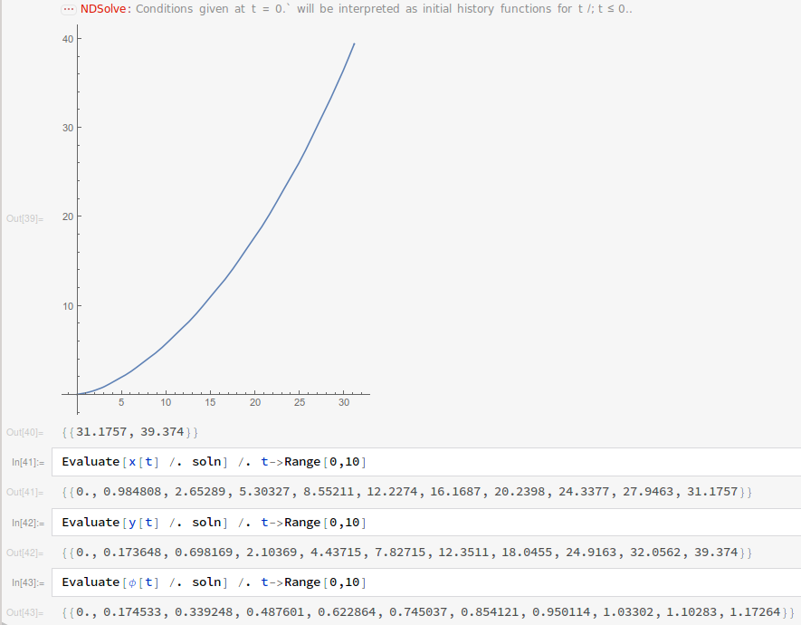
The NDSolve warning is just saying that for tick 0 it doesn’t know what is so it just assumes it’s zero like at (which is fine). We also notice that for is 10 degrees (0.1745 radians). But the solution’s still off… What’s going on at ? The difference difference between the first and second ticks is 9.4366 degrees, not 9.25 degrees like expected. Where did it get that weird number from? The secret lies in looking closer at the individual points being sampled by NDSolve:

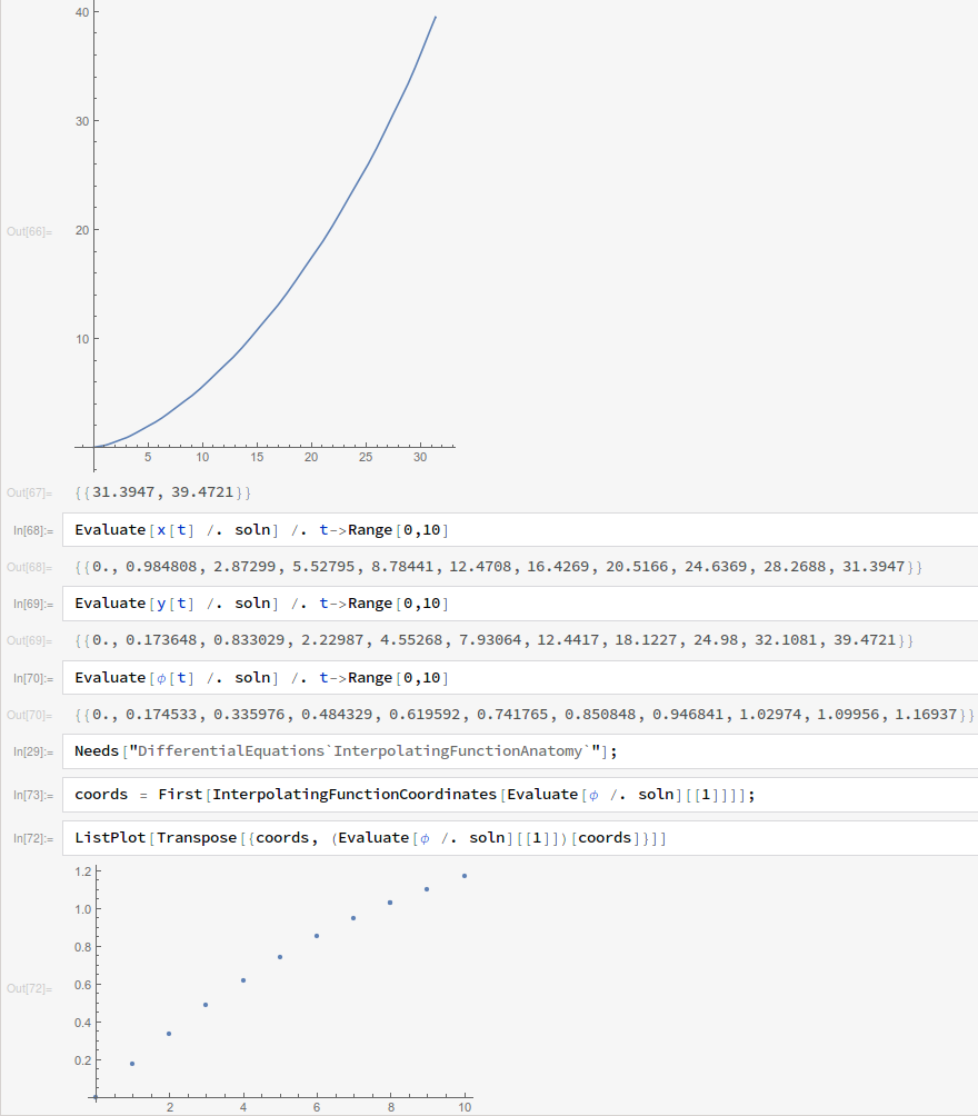
Interesting—between and NDSolve seemed to violate the fixed step guarantee and took half-tick steps, causing the descrepancy between Robocode physics and our Mathematica solution. Further playing around shows that this is caused by the delay differential equation in our dynamics. Luckily, we can reformulate the dynamics to be as follows:

dynamics :=

Module[{vdel=Abs[If[t==0, v[t], v[t]-ta[t]]]}, {

(* Set turn rate to target, but clamp between physical limits *)

veqn = v'[t] == ta[t],

[Phi]eqn = [Phi]'[t] == Clip[t[Omega][t], {-10 Degree + 3/4 Degree * vdel, 10 Degree – 3/4 Degree * vdel}],

xeqn = x'[t] == v[t]Cos[[Phi][t]],

yeqn = y'[t] == v[t]Sin[[Phi][t]]

}]

Which then does the trick and gets us the expected result:

Handling Corner Cases (Try #4)

Although the basic framework is working, there’s still a few corner cases that need to be addressed in order to perfectly match Robocode physics. These include preventing acceleration overshoot (velocity goes from 7.5 to 8.5 and stops there), handling deceleration (two pixels / sec^2), and splitting time between acceleration / deceleration when a tick takes the tank from negative to positive velocity or vice versa. Additionally, there was a weird bug that occured when a WhenEvent fell on the last step of the integration which I fixed by adding a time condition to all the events. I won’t go into the details of finding / fixing the corner cases since it’s just adding a bunch of WhenEvents and corresponding bounds on the initial acceleration. Here’s the finished program, including a range of calculations to show end positions for various and combos:

tEnd = 10; (* Finish time of simulation *)

dynamics :=

Module[{vdel=Abs[If[t==0, v[t], v[t]-ta[t]]]}, {

veqn = v'[t] == ta[t],

(* Set turn rate to target, but clamp between physical limits *)

ϕeqn = ϕ'[t] == Clip[tω[t], {-10 Degree + 3/4 Degree * vdel, 10 Degree – 3/4 Degree * vdel}],

xeqn = x'[t] == v[t]*Cos[ϕ[t]],

yeqn = y'[t] == v[t]*Sin[ϕ[t]]

}]
(* Implicit Euler is not implemented directly, must define ourselves *)

(* Robocode does Implicit Euler for physics *)

ImplicitEuler = {"FixedStep", Method -> {"ImplicitRungeKutta",

"Coefficients" -> "ImplicitRungeKuttaRadauIIACoefficients",

"DifferenceOrder" -> 1, "ImplicitSolver" -> {"FixedPoint",

AccuracyGoal -> MachinePrecision, PrecisionGoal -> MachinePrecision,

"IterationSafetyFactor" -> 1}}};
(* Solves the forward dynamics for an initial state and a target acceleration / turn rate *)

solveDynamics[initialState_, targetAcceleration_, targetTurnRate_, time_] :=

(

(* Add dynamics equations and initial conditions *)

soln = NDSolve[{dynamics, {x[0], y[0], ϕ[0], v[0]}==initialState,

ta[0]==If[v[0]==0, Clip[targetAcceleration, {-1,1}],

If[v[0]+targetAcceleration>0 && v[0]<0, -v[0]+(1+v[0]/2)*1,

If[v[0]+targetAcceleration<0 && v[0]>0, -v[0]-(1-v[0]/2)*1,

(*Else*) Clip[targetAcceleration, {-8-v[0], 8-v[0]}]]]],

tω[0]==targetTurnRate,

(* When velocity reaches zero, start acceleration *)

WhenEvent[Evaluate[v[t]+ta[t]>0 && t!=time], {ta[t]->-v[t]+(1+v[t]/2) * 1}, "DetectionMethod"->"Sign", "LocationMethod"->"StepEnd"],

WhenEvent[Evaluate[v[t]+ta[t]<0 && t!=time], {ta[t]->-v[t]-(1-v[t]/2) * 1}, "DetectionMethod"->"Sign", "LocationMethod"->"StepEnd"],

WhenEvent[Evaluate[v[t]==0 && t!=time], {ta[t]->Clip[targetAcceleration, {-1,1}]}, "DetectionMethod"->"Sign", "LocationMethod"->"StepEnd"],

(* When velocity reaches maximum, stop acceleration *)

WhenEvent[Evaluate[v[t]+ta[t]>8 && t!=time], {ta[t]->8-v[t]}, "DetectionMethod"->"Sign", "LocationMethod"->"StepEnd"],

WhenEvent[Evaluate[v[t]+ta[t]<-8 && t!=time], {ta[t]->-8-v[t]}, "DetectionMethod"->"Sign", "LocationMethod"->"StepEnd"],

WhenEvent[Evaluate[v[t]*Sign[targetAcceleration]==8 && t!=time], {ta[t]->0}, "DetectionMethod"->"Sign", "LocationMethod"->"StepEnd"]},

(* Specify desired outputs and integration timeframe *)

{x, y, x’, y’, v, ϕ, ϕ’, ta, tω}, {t, 0, time},

(* Allow target turn / accelerate variables to jump discontinuously *)

DiscreteVariables->{tω, ta},

(* Use a ImplicitEuler method with a step size of one tic (matches robocode) *)

StartingStepSize->1, Method->ImplicitEuler];

Flatten[{x[time], y[time], ϕ[time], v[time]} /. soln]

)
(* Plot various end positions starting from rest *)

zeroVelSoln = Flatten[Table[solveDynamics[{0,0,0,0}, a, ω, tEnd], {a, -1, 1, 0.1}, {ω, -10 Degree, 10 Degree, 1 Degree}], 1];

zvxysoln = Part[#, {1,2}]& /@ zeroVelSoln;

ListPlot[zvxysoln, AxesLabel->{Subscript[x, final],Subscript[y, final]}]
(* Plot the extreme positions for a range of initial velocities as a point cloud *)

solnA = Flatten[Table[Join[solveDynamics[{0, 0, 0, vi}, a, ω, tEnd], {vi}], {vi, 8, 8, 16}, {a, -2, 1, 0.1}, {ω, -10 Degree, 10 Degree, 1 Degree}], 2];

solnB = Flatten[Table[Join[solveDynamics[{0, 0, 0, vi}, a, ω, tEnd], {vi}], {vi, -8, -8, 16}, {a, -1, 2, 0.1}, {ω, -10 Degree, 10 Degree, 1 Degree}], 2];

solnC = Flatten[Table[Join[solveDynamics[{0, 0, 0, vi}, a, ω, tEnd], {vi}], {vi, -7, 0, 1}, {a, -1, 2, 3}, {ω, -10 Degree, 10 Degree, 1 Degree}], 2];

solnD = Flatten[Table[Join[solveDynamics[{0, 0, 0, vi}, a, ω, tEnd], {vi}], {vi, -7, 0, 1}, {a, -1, 2, 0.1}, {ω, -10 Degree, 10 Degree, 20 Degree}], 2];

solnE = Flatten[Table[Join[solveDynamics[{0, 0, 0, vi}, a, ω, tEnd], {vi}], {vi, 0, 7, 1}, {a, -2, 1, 3}, {ω, -10 Degree, 10 Degree, 1 Degree}], 2];

solnF = Flatten[Table[Join[solveDynamics[{0, 0, 0, vi}, a, ω, tEnd], {vi}], {vi, 0, 7, 1}, {a, -2, 1, 0.1}, {ω, -10 Degree, 10 Degree, 20 Degree}], 2];

soln = Join[solnA, solnB, solnC, solnD, solnE, solnF];

xysoln = Part[#, {1,2,5}]& /@ soln;

ListPointPlot3D[xysoln, AxesLabel->{Subscript[x, final],Subscript[y, final],Subscript[v, initial]}]

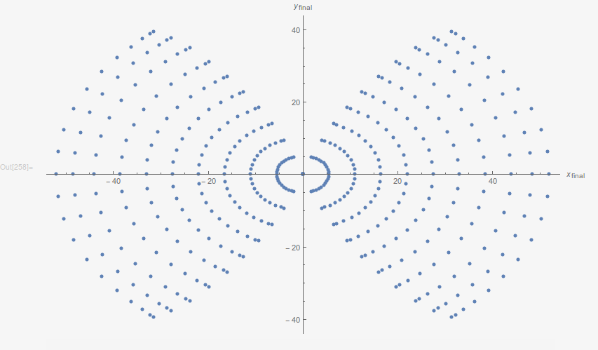
In the second graph, the points in each horizontal slice represent the extreme possible positions of one specific starting velocity (essentially the boundary points of the previous graph). When these are stacked on top of each other over a range of possible initial velocities, this interesting 3D shape is the result.

Takeaways

Here’s a few general remarks about my experience using Mathematica to integrate discrete-time ODEs:

• Implicit Euler integration, while not supported by default, can be fairly easily defined by the user
• Inequality constraints can be formulated using WhenEvents (just take care to address overshoots and clip the initial conditions appropriately)
• Specifying “LocationMethod” on WhenEvents to match the integration scheme may be necessary
• Delay differential equations can cause NDSolve to violate a FixedStep integration method–try to reformulate the equations if possible
• Strange WhenEvent behavior on the final integration step can be avoided by adding a time condition

I used Mathematica 11.0.1.0 for this project–later versions may fix some of the problems I encountered. This was also my first time working with Mathematica so don’t take my code as any kind of style guide. Regardless, I hope you can use some of my experiences to debug your own NDSolve issues.