Numerical methods for trajectory optimization have become increasingly popular for analyzing the motion of bipedal spring-mass walkers, whose complex nonlinear dynamics make analytical solutions often infeasible. When I began looking into trajectory optimization, the number of different methods often obscured some of the basic ideas in the field. This tutorial is meant to provide a simple introduction to trajectory optimization with some example code and references for further reading.
Function Optimization
The core of trajectory optimization is constrained function optimization. In this tutorial, I use Matlab’s fmincon—alternatives include SNOPT and IPOPT. In simple terms, fmincon finds the set of parameters that minimize a certain objective function, subject to linear or nonlinear constraints. These constraints can be formulated in four different ways, as documented at the above link: linear equality, linear inequality, nonlinear equality, and nonlinear inequality. Let’s illustrate a possible application of this with a short example (taken from Minoj Srinivasan’s lecture slides).
Say there’s a target at the coordinates [5, 10]. We want to shoot a cannon ball at the target from position [0, 0], minimizing the amount of initial energy required (proportional to  ). The optimizer controls three parameters:
  ,
,  , and the flight time. The only constraint is that after flying for the designated time with the given initial conditions the cannon ball must end up close to the target (how close is a parameter to the optimizer). We lower bound the simulation time at zero and give it an initial guess for the appropriate parameters.
flight.m
% The function to be minimized (E = vx_0^2 + vy_0^2)
energy_fun = @(x) (x(2)^2 + x(3)^2);

% The initial parameter guess; time = 1; vx_0 = 2, vy_0 = 3
x0 = [1; 2; 3];
% No linear inequality or equality constraints
A = [];
b = [];
Aeq = [];
Beq = [];
% Lower bound the simulation time at zero, leave initial velocities unbounded
lb = [0; -Inf; -Inf];
ub = [Inf; Inf; Inf];
% Solve for the best simulation time + control input
optimal = fmincon(energy_fun, x0, A, b, Aeq, Beq, lb, ub, ...
                  @flight_constraint, options);
% Unpack the parameters
opt_time = optimal(1);
opt_vx0 = optimal(2);
opt_vy0 = optimal(3);

fprintf('Optimal time: %f\n', opt_time);
fprintf('Optimal initial velocity: [%f, %f]\n', opt_vx0, opt_vy0);
flight_constraint.m
function [ c, ceq ] = flight_constraint( x )
    c = [];
    % Unpack the parameters
    time = x(1);
    vx_0 = x(2);
    vy_0 = x(3);
    % Calculate the travel distances
    x_travel = time * vx_0;
    y_travel = time * vy_0 - 0.5 * 9.81 * time^2;
    % The following two constraints must equal zero, meaning that the
    % target is set at x = 5 and y = 10
    ceq = [x_travel - 5; y_travel - 10];
end
Trajectory Optimization with Time-Dependent Control Input
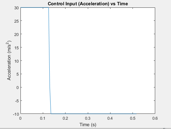
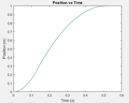
In the previous example, the optimizer could only adjust the initial conditions of the cannon ball and the flight time. What if we want to find an optimal trajectory with a control input that varies with time? The trick here is to discretize the control input into n segments and include each segment as a variable in the parameter vector. Let’s consider an example of this strategy applied to the canonical double-integrator (state is position and velocity along line, control input is acceleration). The control input is the second derivative of the position, and the constraints specify that the final position should be one and the final velocity should be zero. Our parameter vector consists of the simulation time followed by one hundred time-discretized accelerations. The optimizer is instructed to find the minimum time solution.
double_integrator.m
% Minimize the simulation time
time_min = @(x) x(1);
% The initial parameter guess; 1 second, with a hundred accelerations
% all initialized to 5
x0 = [1; ones(100, 1) * 5];
% No linear inequality or equality constraints
A = [];
b = [];
Aeq = [];
Beq = [];
% Lower bound the simulation time at zero seconds, and bound the
% accelerations between -10 and 30
lb = [0; ones(100, 1) * -10];
ub = [Inf; ones(100, 1) * 30];
% Options for fmincon
options = optimset('TolFun', 0.00000001, 'MaxIter', 100000, ...
'MaxFunEvals', 100000);
% Solve for the best simulation time + control input
optimal = fmincon(time_min, x0, A, b, Aeq, Beq, lb, ub, ...
@double_integrator_constraints, options);
% The simulation time is the first element in the solution
sim_time = optimal(1);
% The time discretization
delta_time = sim_time / (length(optimal) - 1);
times = 0 : delta_time : sim_time - delta_time;
% The accelerations given by the optimizer
accs = optimal(2:end);
% The resulting velocities (integrate accelerations with respect to time)
vels = cumtrapz(times, accs);
% The resulting positions (integrate velocities with respect to time)
positions = cumtrapz(times, vels);
% Make the plots
figure();
plot(times, accs);
title('Control Input (Acceleration) vs Time');
xlabel('Time (s)');
ylabel('Acceleration (m/s^2)');
figure();
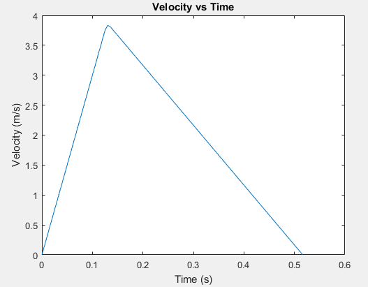
plot(times, vels);
title('Velocity vs Time');
xlabel('Time (s)');
ylabel('Velocity (m/s)');
figure();
plot(times, positions);
title('Position vs Time');
xlabel('Time (s)');
ylabel('Position (m)');
double_integrator_constriants.m
function [ c, ceq ] = double_integrator_constraints( x )
    % No nonlinear inequality constraint needed
    c = [];
    % Discretize the times into a vector
    sim_time = x(1);
    delta_time = sim_time / (length(x) - 1);
    times = 0 : delta_time : sim_time - delta_time;
    % Get the accelerations out of the rest of the parameter vector
    accs = x(2:end);
    % Integrate up the velocities and final position
    vels = cumtrapz(times, accs);
    pos = trapz(times, vels);
    % All elements of this vector must be constrained to equal zero
    % This means that final pos must equal 1 (target) and the end velocity
    % must be equal to zero.
    ceq = [pos - 1; vels(end)];
end
As we can see from the graphs, the optimizer logically found bang-bang control to be optimal. Additionally, note that the fraction of time spent in either max-acceleration or min-acceleration is corresponds to the ratio of the max/min bounds. Intuitively, this provides the fastest trajectory while still satisfying the zero-end-velocity constraint.
A Note on Single Shooting vs Multiple Shooting
The trajectory optimization method detailed above is known as “single shooting.” This means that we simulate the whole trajectory and try to drive the deviation of the endpoint to zero. Multiple shooting is slightly more sophisticated—instead of simulating the whole trajectory at once, the trajectory is broken apart into multiple subintervals. For each subinterval, the starting position is added as a parameter and a constraint is added suchthat the deviation between the end of one subinterval and the beginning of another must end up being zero. This approach enables the optimizer to solve much more complex problems than with single shooting.
Further Reading
I hope this article was helpful for better understanding trajectory optimization! Please keep in mind that this is just a tutorial to get you started with some of the basic concepts, and I highly encourage you to check out the references below:
- Overview of various transcription methods: http://www.matthewpeterkelly.com/research/MattKelly__Transcription_Methods_for_Trajectory_Optimization.pdf
- Interesting examples of trajectory optimization: http://www.cs.cmu.edu/~cga/dynopt/readings/trajopt2.pdf
- Powerpoint for the cannon example: http://movement.osu.edu/software/DW2010/TrajOptim_ManojSrinivasan2010.pdf
Leave a Reply