Optimizing Trajectories for the Spring Loaded Inverted Pendulum over Slippery Terrain

Previously, I’ve written short introductions to numerical trajectory optimization here and here—if you’re unfamiliar with the basics, I recommend you check those out first.

This write up expands upon a section of my research paper (which I hope to finish soon) and is meant to be a walkthrough of how to apply numerical trajectory optimization to real-world scenarios.

The Problem

The Spring Loaded Inverted Pendulum (SLIP) model is often used to approximate human running dynamics. Fundamentally, SLIP hoppers represent the mass of the torso as a point at the hip and connect the hip to the foot via a spring. In other words, the biped becomes a pogo stick, bouncing from foot to foot with each step.

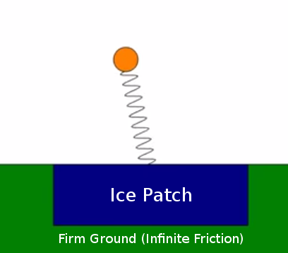
We consider the case where a running planar biped steps on an unforeseen ice patch, surrounded with high-friction ground on each side. The question then becomes this: should the robot attempt to use its momentum to traverse the patch in one step, or first step backwards and then launch itself over the patch to the other side?

Modified SLIP

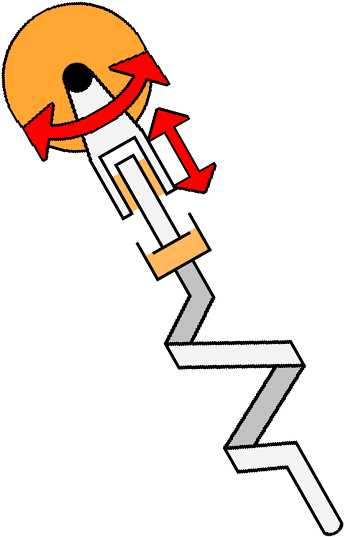
In addition to the basic SLIP model, I included a few modifications:

Damper in series with spring
Hip torque actuation
Second derivative of neutral length actuation
Foot mass (for sliding)

The SLIP model used in the optimization.

SLIP Dynamics

Before constructing the optimization problem, we need to know the dynamics of the system. A “phase” represents a section of a trajectory with continuous state and one set of governing equations. Three different types of phases are possible in this system: standing on ground, slipping on ice, and flying through the air. Since the first two cases are similar, we will first handle them together and then discuss flight phases.

Stance Phase

Let ( $x$ , $y$ ) be the hip position, $x_{toe}$ be the toe horizontal position, $k$ be the spring coefficient, $c$ be the damping coefficient, $r$ be the SLIP length, $r_a$ be the actuated SLIP length (or neutral spring length), $\tau$ be the hip torque, $m_{hip}$ and $m_{toe}$ be the hip and toe masses, respectively, and $g$ be the gravitational constant. The state of the SLIP can be then represented as follows:

$X = \begin{bmatrix}x_{toe} \\\dot{x_{toe}} \\ x \\ \dot{x} \\ y \\ \dot{y} \\ r_a \\ \dot{r_a} \end{bmatrix}$

And the SLIP length $r$ can then be written as:

(1) $\begin{equation*} r = \sqrt{(x-x_{toe})^2 + y^2} \end{equation*}$

Differentiating by the chain rule, we get the following equation for the time derivative of $r$ :

(2) $\begin{equation*} \dot{r} = \frac{(x-x_{toe}) \cdot (\dot{x} - \dot{x_{toe}}) + y\dot{y}}{r} \end{equation*}$

The force exerted by the spring-damper combination can then be expressed as follows:

(3) $\begin{equation*} F_s = k(r_a - r) + c(\dot{r_a} - \dot{r}) \end{equation*}$

While the force exerted by the hip torque on the ground is simply:

(4) $\begin{equation*} F_t = \frac{\tau}{r} \end{equation*}$

Realizing that the cosine of the angle between the SLIP and the ground is equal to $\frac{x-x_{toe}}{r}$ and the sine is equal to $\frac{y}{r}$ , it is possible to express the acceleration of the hip:

(5) $\begin{equation*} \ddot{x} = \frac{1}{m_{hip}} \cdot (F_s \frac{x-x_{toe}}{r} + F_t \frac{y}{r}) \end{equation*}$

(6) $\begin{equation*} \ddot{y} = \frac{1}{m_{hip}} \cdot (F_s\frac{y}{r} - F_t\frac{x-x_{toe}}{r} - m_{hip} \cdot g) \end{equation*}$

However, it is also necessary to know the acceleration of the toe on the ice. We first determine the ground reaction force as follows:

(7) $\begin{equation*} GRF = F_s\frac{y}{r} - F_t\frac{x-x_{toe}}{r} + m_{toe}g \end{equation*}$

The force of friction on the toe is then given as:

(8) $\begin{equation*} F_f = -\mu \cdot \tanh(50\dot{x_{toe}}) \cdot GRF \end{equation*}$

Where the $\tanh(50\dot{x_{toe}})$ serves as a smooth approximation of a sign function, whose discontinuities create convergence difficulties for the optimizer.
Finally, the acceleration of the toe can be expressed as follows:

(9) $\begin{equation*} \ddot{x_{toe}} = \begin{cases} 0 & \text{stick phase} \\ \frac{1}{m_{toe}} \cdot (-F_s\frac{x-x_{toe}}{r} - F_t\frac{y}{r} + F_f) & \text{slip phase} \\ \end{cases} \end{equation*}$

This concludes the SLIP dynamics during both slippery and high-friction stance phases.

Flight Phase

Flight phases are governed by the standard equations for ballistic trajectories and are triggered when the ground reaction force intersects zero. First, we declare a free variable, $t_{flight}$ . The following equations then result:

$x_{land} = x_{to} + \dot{x}_{to} t_{flight}$

$y_{land} = y_{to} + \dot{y}_{to} t_{flight} - \frac{g \cdot t_{flight}^2}{2}$

Where all “to” subscripts represent takeoff states and all “land” subscripts represent landing states.

Formulating constraints

Within a certain phase, constraints are formulated using direct collocation, which discretizes the states and control inputs at evenly-spaced nodes and enforces the dynamics between nodes using hard equality constraints. The following inequality constraints are also enforced at every node:

$r < r_{max}$
$r > r_{min}$
- The ground reaction force must be positive within a phase for ground contact to occur. The only exceptions are the last nodes of stance phases that have a flight phase following them (instead are equality constrained to zero). The last node of the last phase, however, does need the GRF inequality constraint.
- Prevents unreasonably large GRF forces that might damage the robot.

There also need to be constraints governing phase transitions. Since the flight dynamics are solvable in closed form, this ultimately amounts to linking the end of one stance phase to the beginning of the next in a way which obeys the flight dynamics. Discretizing the state along the flight path is unnecessary.

As mentioned previously, the flight time parameter $t_{flight}$ here is really critical. I first fooled around with a bunch of different strategies (for example parameterizing a completely separate landing state, with the landing angle and length inferred from the first node of the next phase, and then equality constraining the two). None converged reliably; many thanks to Christian Hubicki for pointing me in the right direction here.

The best method turned out to be evaluating the end state of the ballistic flight trajectory from the take off state and flight time, and then equality constraining that with the first node of the next stance phase. The specific variables that were constrained from the flight phase were $x$ , $\dot{x}$ , $y$ , $\dot{y}$ , and $\dot{x_{toe}} = \dot{x}$ . The ground reaction force at takeoff and $\dot{r_a}$ at touchdown are constrained to zero, and $r_a$ is constrained equal to $r$ at touchdown.

There are a few more variables and constraints that are important to note. Each stance and flight phase had a time parameter, which was bounded using the lower bound and upper bound arguments to fmincon. Similarly, the max/min actuated leg length second derivative and hip torque were also bounded in the fmincon bounds arguments. The toe x position was bounded to be within the ice patch for the slippery phase and outside for the sticky phase. The initial SLIP state was constrained to a starting position over the ice patch, and the final SLIP x and toe x were constrained to be slightly to the right of the ice patch.

Objective functions

Cold-initializing an energy-optimizing objective with random parameters often results in failure to converge due to the large number of parameters and constraints. Therefore, a three-step optimization was used:

Constant objective function (find any trajectory which satisfies constraints)
Resulting trajectory is fed into impulse cost function:
(10) $\begin{equation*} C_{imp} = \sum_{n=1}^{N_{phase}} \sum_{i=1}^{N_{grid}} [(\ddot{r_a}_{n,i} \cdot \Delta t_n)^2 + (\tau_{n,i} \cdot \Delta t_n)^2] \end{equation*}$

Where $N_{phase}$ is the number of stance phases, $N_{grid}$ is the number of discretization nodes per stance phase, and $\Delta t_n$ is equal to the n_th stance phase time $T_n$ divided by $N_{grid}$ .
Output trajectory of impulse cost function is fed into work cost function:
(11) $\begin{equation*} \sum_{n=1}^{N_{phase}} \bigg[\int_{0}^{T_n} |F_s \cdot \dot{r_a}|dt + \int_{\theta_{td}}^{\theta_{to}}|\tau d\theta|\bigg] \end{equation*}$

Since the absolute value function is inherently nonsmooth—creating optimizer convergence problems—a smooth approximation was employed:

(12) $\begin{equation*} |x| \approx \sqrt{x^2 + \epsilon^2} - \epsilon \end{equation*}$

Where $\epsilon$ is about $10^{-3}$ .

Problem Formulation

As mentioned previously, the trajectory optimization problem was transcribed using direct collocation with 10 nodes per stance phase. For linking one node to the next within a stance phase, dynamics were integrated using trapezoidal quadrature. Matlab’s fmincon was used for the optimization, with the SQP algorithm specified. Jacobians were symbolically calculated to accelerate convergence. The whole three-step optimization takes on the order of a few minutes to complete and converges reliably from random initial parameters.

Code

main.m

GEN_CONSTRAINTS = true;
GEN_COSTS = true;

sp = SimParams(['str'], [0,1], [1.1; 0; 1.1-cosd(45); 0; ...
                                sind(45); 0; 1; 0], 1.1);

% Options for optimizing the constant cost function
cOptions = optimoptions(@fmincon, 'TolFun', 0.00000001, ...
                       'MaxIterations', 100000, ...
                       'MaxFunEvals', 50000, ...
                       'Display', 'iter', 'Algorithm', 'sqp', ...
                       'StepTolerance', 1e-13, ...
                       'SpecifyConstraintGradient', true, ...
                       'SpecifyObjectiveGradient', true, ...
                       'ConstraintTolerance', 1e-6, ...
                       'CheckGradients', false, ...
                       'HonorBounds', true, ...
                       'FiniteDifferenceType', 'forward');
% Options for optimizing the actual cost function
aOptions = optimoptions(@fmincon, 'TolFun', 0.00000001, ...
                       'MaxIterations', 1000, ...
                       'MaxFunEvals', 1000000, ...
                       'Display', 'iter', 'Algorithm', 'sqp', ...
                       'StepTolerance', 1e-13, ...
                       'SpecifyConstraintGradient', true, ...
                       'SpecifyObjectiveGradient', true, ...
                       'ConstraintTolerance', 1e-6, ...
                       'CheckGradients', false, ...
                       'HonorBounds', true, ...
                       'FiniteDifferenceType', 'forward');
% No linear inequality or equality constraints
A = [];
B = [];
Aeq = [];
Beq = [];
% Set up the bounds
[lb, ub] = bounds(sp);

tic

numVars = size(sp.phases, 1) * 2 - 1 + sp.gridn * size(sp.phases, 1) * 10;
funparams = conj(sym('x', [1 numVars], 'real')');

if GEN_CONSTRAINTS
    fprintf('Generating constraints...\n');
    [c, ceq] = constraints(funparams, sp);
    cjac = jacobian(c, funparams).';
    ceqjac = jacobian(ceq, funparams).';
    constraintsFun = matlabFunction(c, ceq, cjac, ceqjac, 'Vars', {funparams});
    fprintf('Done generating constraints...\n');
end

if GEN_COSTS
    fprintf('Generating costs...\n');
    ccost = constcost(funparams, sp);
    ccostjac = jacobian(ccost, funparams).';
    ccostFun = matlabFunction(ccost, ccostjac, 'Vars', {funparams});

    acost = actsqrcost(funparams, sp);
    acostjac = jacobian(acost, funparams).';
    acostFun = matlabFunction(acost, acostjac, 'Vars', {funparams});
    
    awcost = actworkcost(funparams, sp);
    awcostjac = jacobian(awcost, funparams).';
    awcostFun = matlabFunction(awcost, awcostjac, 'Vars', {funparams});
    fprintf('Done generating costs...\n');
end

flag = -1;
tryCount = 0;
while flag < 0 && tryCount < 3
    fprintf('Generating initial possible trajectory (%d)...\n', tryCount+1);
    % Generate initial guess
    x0 = MinMaxCheck(lb, ub, ones(numVars, 1) * rand() * 2);
    [ci, ceqi, cjaci, ceqjaci] = constraintsFun(x0);
    while any(imag(ci))  || any(imag(ceqi))  || any(any(imag(cjaci)))  || any(any(imag(ceqjaci)))  || ...
          any(isnan(ci)) || any(isnan(ceqi)) || any(any(isnan(cjaci))) || any(any(isnan(ceqjaci))) || ...
          any(isinf(ci)) || any(isinf(ceqi)) || any(any(isinf(cjaci))) || any(any(isinf(ceqjaci)))
        fprintf('Regenerating initial guess...\n');
        x0 = MinMaxCheck(lb, ub, ones(numVars, 1) * rand());
        [ci, ceqi, cjaci, ceqjaci] = constraintsFun(x0);
    end

    % Find any feasible trajectory
    [feasible, ~, flag, ~] = ...
        fmincon(@(x) call(ccostFun, x, 2),x0,A,B,Aeq,Beq,lb,ub, ...
                @(x) call(constraintsFun, x, 4), cOptions);
    tryCount = tryCount + 1;
end

if flag > 0
    fprintf('Optimizing for torque/raddot squared...\n');
    % Optimize for torque/raddot squared cost
    [optimal, ~, ~, ~] = ...
        fmincon(@(x) call(acostFun, x, 2),feasible,A,B, ...
                Aeq,Beq,lb,ub,@(x) call(constraintsFun,x,4),aOptions);
    fprintf('Optimizing for work...\n');
    % Optimize for minimum work
    [optimal, cost, flag, ~] = ...
        fmincon(@(x) call(awcostFun, x, 2),optimal,A,B, ...
                Aeq,Beq,lb,ub,@(x) call(constraintsFun,x,4),aOptions);
    fprintf('Done optimizing\n');
else
    optimal = [];
    cost = 0;
    fprintf('Exited with non-positive flag: %d\n', flag);
end

fprintf('Finished optimizing in %f seconds\n', toc);

constraints.m

function [ c, ceq ] = constraints( funparams, sp )
    % Phase inequality constraints
    phaseIC = sym('pic', [1, 4*sp.gridn*size(sp.phases, 1)])';
     
    % Phase equality constraints
    phaseEC = sym('pec', [1, 8*(sp.gridn-1)*size(sp.phases, 1)])';
    % Phase transition equality constraints
    transEC = sym('tec', [1, 8*(size(sp.phases, 1)-1)])';
    
    % Unpack the parameter vector
    [ stanceT, flightT, xtoe, xtoedot, x, xdot, y, ydot, ...
           ra, radot, raddot, torque] = unpack(funparams, sp);
    
    % Iterate over all the phases
    for p = 1 : size(sp.phases, 1)
        phaseStr = sp.phases(p, :);
        % The index of the first dynamics variable for the current phase
        ps = (p - 1) * sp.gridn + 1;
        
        % Calculate the timestep for that specific phase
        dt = stanceT(p) / sp.gridn;
        
        % Take off state at the end of the last phase
        if p > 1
            toState = stateN;
            toCompvars = compvarsN;
        end
        
        stateN = [xtoe(ps); xtoedot(ps); x(ps);  xdot(ps);   ...
                  y(ps);    ydot(ps);    ra(ps); radot(ps)];
        
        % Link ballistic trajectory from end of last phase to this phase
        if p > 1
            rland = sqrt((x(ps) - xtoe(ps))^2 + y(ps)^2);
            
            [xtoedotland, xland, xdotland, yland, ydotland] = ...
                ballistic(toState, flightT(p-1), sp, phaseStr);
            % Grf must equal zero at takeoff
            transEC((p-2)*8+1 : (p-1)*8) = ...
                    [xtoedotland-xtoedot(ps); xland-x(ps); ...
                    xdotland-xdot(ps); yland-y(ps); ydotland-ydot(ps); ...
                    ra(ps) - rland; radot(ps); toCompvars.grf];
        end
            
        % Offset in the equality parameter vector due to phase
        pecOffset = 8 * (sp.gridn - 1) * (p - 1);
        % Offset in the inequality parameter vector due to phase
        picOffset = 4 * (sp.gridn) * (p - 1);
        
        [statedotN, compvarsN] = dynamics(stateN, raddot(ps), ...
                                          torque(ps), sp, phaseStr);
        for i = 1 : sp.gridn - 1
            % The state at the beginning of the time interval
            stateI = stateN;
            % What the state should be at the end of the time interval
            stateN = [xtoe(ps+i); xtoedot(ps+i); x(ps+i);  xdot(ps+i); ...
                      y(ps+i);    ydot(ps+i);    ra(ps+i); radot(ps+i)];
            % The state derivative at the beginning of the time interval
            statedotI = statedotN;
            % Some calculated variables at the beginning of the interval
            compvarsI = compvarsN;
            % The state derivative at the end of the time interval
            [statedotN, compvarsN] = ...
                dynamics(stateN, raddot(ps+i), torque(ps+i), sp, phaseStr);

            % The end position of the time interval calculated using quadrature
            endState = stateI + dt * (statedotI + statedotN) / 2;
            
            % Constrain the end state of the current time interval to be
            % equal to the starting state of the next time interval
            phaseEC(pecOffset+(i-1)*8+1:pecOffset+i*8) = stateN - endState;
            % Constrain the length of the leg, grf, and body y pos
            phaseIC(picOffset+(i-1)*4+1 : picOffset+i*4) = ...
                    [compvarsI.r - sp.maxlen; sp.minlen - compvarsI.r; ...
                     -compvarsI.grf; compvarsI.grf - sp.maxgrf];
        end
        
        if p == size(sp.phases, 1)
            % Constrain the length of the leg at the end position
            % Since it's the end of the last phase, add grf constraint
            phaseIC(picOffset+(sp.gridn-1)*4+1:picOffset+sp.gridn*4) = ...
                [compvarsN.r - sp.maxlen; sp.minlen - compvarsN.r; ...
                -compvarsN.grf; compvarsN.grf - sp.maxgrf];
        else 
            % Constrain the length of the leg at the end position
            % No ground reaction force constraint (this will be handled in
            % transition equality constraints)
            phaseIC(picOffset+(sp.gridn-1)*4+1:picOffset+sp.gridn*4) = ...
                [compvarsN.r - sp.maxlen; sp.minlen - compvarsN.r; -1; -1];
        end
    end
    
    c = phaseIC;
    ceq = [phaseEC; transEC];
    
    initialState = [xtoe(1); xtoedot(1); x(1);  xdot(1);   ...
                  y(1);    ydot(1);    ra(1); radot(1)];
              
    % Add first phase start constraints
    ceq = [ceq; initialState - sp.initialState];
    % Add last phase end constraints
    ceq = [ceq; x(end) - sp.finalProfileX; xtoe(end) - sp.finalProfileX];
end

unpack.m

function [ stanceT, flightT, xtoe, xtoedot, x, xdot, y, ydot, ...
           ra, radot, raddot, torque] = unpack( funparams, sp )
    p = size(sp.phases, 1);
    cnt = sp.gridn * p;
    
    stanceT       = funparams(1               : p);
    flightT       = funparams(p + 1           : p * 2 - 1);
    xtoe          = funparams(p * 2           : p * 2 - 1 + cnt);
    xtoedot       = funparams(p * 2 + cnt     : p * 2 - 1 + cnt * 2);
    x             = funparams(p * 2 + cnt * 2 : p * 2 - 1 + cnt * 3);
    xdot          = funparams(p * 2 + cnt * 3 : p * 2 - 1 + cnt * 4);
    y             = funparams(p * 2 + cnt * 4 : p * 2 - 1 + cnt * 5);
    ydot          = funparams(p * 2 + cnt * 5 : p * 2 - 1 + cnt * 6);
    ra            = funparams(p * 2 + cnt * 6 : p * 2 - 1 + cnt * 7);
    radot         = funparams(p * 2 + cnt * 7 : p * 2 - 1 + cnt * 8);
    raddot        = funparams(p * 2 + cnt * 8 : p * 2 - 1 + cnt * 9);
    torque        = funparams(p * 2 + cnt * 9 : p * 2 - 1 + cnt * 10);
end

dynamics.m

function [ statedot, compvars ] = dynamics( state, raddot, torque, sp, curPhase )
    stateCell = num2cell(state');
    [xtoe, xtoedot, x, xdot, y, ydot, ra, radot] = deal(stateCell{:});
    
    r = sqrt((x - xtoe)^2 + y^2);
    rdot = ((x-xtoe)*(xdot-xtoedot)+y*ydot)/(r);
    cphi = (x-xtoe) / r;
    sphi = y / r;
    fs = sp.spring * (ra - r) + sp.damp * (radot - rdot);
    ft = torque / r;
    fg = sp.masship * sp.gravity;

    xddot = (1/sp.masship) * (fs*cphi + ft * sphi);
    yddot = (1/sp.masship) * (fs*sphi + ft * (-cphi) - fg);

    grf = fs * sphi - ft * cphi + sp.masstoe * sp.gravity;

    % Check if the phase should be slipping
    if strcmp(curPhase, 'sli')
        ff = -sp.friction * tanh(xtoedot * 50) * grf;
        xtoeddot = (1/sp.masstoe) * (-fs*cphi - ft*sphi + ff);
    else
        xtoeddot = 0;
    end

    statedot = [xtoedot; xtoeddot; xdot; xddot; ydot; yddot; ...
                radot; raddot];

    compvars.r = r;
    compvars.grf = grf;
end

ballistic.m

function [ xtoedotland, xland, xdotland, yland, ydotland ] = ...
        ballistic( toState, flightTime, sp, curPhase )

    stateCell = num2cell(toState');
    [~, ~, x, xdot, y, ydot, ~, ~] = deal(stateCell{:});

    if strcmp(curPhase, 'sli')
        xtoedotland = xdot;
    else
        xtoedotland = 0;
    end
    xland = x + xdot * flightTime;
    yland = y + ydot * flightTime - 0.5 * sp.gravity * flightTime^2;
    xdotland = xdot;
    ydotland = ydot - sp.gravity * flightTime;
end

constcost.m

function [ cost ] = constcost( funparams, sp )
    cost = sym(1);
end

actsqrcost.m

function [ cost ] = actsqrcost( funparams, sp )
    % Unpack the vector
    [stanceT, ~, ~, ~, ~, ~, ~, ~, ~, ~, raddot, torque] = ...
        unpack(funparams, sp);

    dts = kron(stanceT./sp.gridn, ones(sp.gridn, 1));
    cost = sum((raddot .* dts) .^ 2) + sum((torque .* dts) .^ 2);
end

actworkcost.m

function [ cost ] = actworkcost( funparams, sp )
    % Unpack the vector
    [stanceT, ~, xtoe, ~, x, xdot, y, ydot, ra, radot, ~, torque] = ...
        unpack(funparams, sp);
    phaseN = size(sp.phases, 1);
    
    r = sqrt((x - xtoe).^2 + y.^2);
    rdot = ((x-xtoe).*(xdot)+y.*ydot)./(r);
    fs = sp.spring * (ra - r) + sp.damp * (radot - rdot);
    
    startRemInd = 1 : sp.gridn : sp.gridn * phaseN;
    endRemInd = sp.gridn : sp.gridn : sp.gridn * phaseN;
    
    [fsA, fsB] = deal(fs);
    fsA(startRemInd) = [];
    fsB(endRemInd) = [];
    fsCombined = (fsA + fsB) .* 0.5;
    
    [radotA, radotB] = deal(radot);
    radotA(startRemInd) = [];
    radotB(endRemInd) = [];
    radotCombined = (radotA + radotB) .* 0.5;
    
    epsilon = 0.001;
    workRa = (sqrt((fsCombined.*radotCombined).^2 + epsilon^2) - epsilon);
    workRa = workRa .* kron(stanceT./sp.gridn, ones(sp.gridn - 1, 1));
    
    angles = atan2(y, x - xtoe);
    angleShift = [angles(1); angles(1 : end-1)];
    angleDeltas = angles - angleShift;
    angleDeltas(startRemInd) = [];
    [torqueA,torqueB] = deal(torque);
    torqueA(startRemInd) = [];
    torqueB(endRemInd) = [];
    torqueCombined = (torqueA + torqueB) .* 0.5;
    
    workAng = sqrt((torqueCombined.*angleDeltas).^2 + epsilon^2) - epsilon;
    cost = sum(workRa) + sum(workAng);
end

bounds.m

function [ lb, ub ] = bounds(sp)
    stanceTimeMin      = sp.minStanceTime;
    stanceTimeMax      = sp.maxStanceTime;
    flightTimeMin      = sp.minFlightTime;
    flightTimeMax      = sp.maxFlightTime;
    minXtoedot         = -Inf;
    maxXtoedot         = Inf;
    minX               = -Inf;
    maxX               = Inf;
    minXdot            = -Inf;
    maxXdot            = Inf;
    minY               = 0;
    maxY               = Inf;
    minYdot            = -Inf;
    maxYdot            = Inf;
    minRa              = -Inf;
    maxRa              = Inf;
    minRadot           = -Inf;
    maxRadot           = Inf;
    minRaddot          = sp.minraddot;
    maxRaddot          = sp.maxraddot;
    minTorque          = sp.mintorque;
    maxTorque          = sp.maxtorque;

    minXtoe = [];
    maxXtoe = [];

    for p=1:size(sp.phases, 1)
        phase = sp.phases(p, :);
        if strcmp(phase, 'sli')
            minXtoe = [minXtoe; ones(sp.gridn, 1) * sp.slipPatch(1)];
            maxXtoe = [maxXtoe; ones(sp.gridn, 1) * sp.slipPatch(2)];
        elseif strcmp(phase, 'stl')
            minXtoe = [minXtoe; ones(sp.gridn, 1) * -Inf];
            maxXtoe = [maxXtoe; ones(sp.gridn, 1) * sp.slipPatch(1)];
        elseif strcmp(phase, 'str')
            minXtoe = [minXtoe; ones(sp.gridn, 1) * sp.slipPatch(2)];
            maxXtoe = [maxXtoe; ones(sp.gridn, 1) * Inf];
        end
    end

    stanceTimeVars = ones(size(sp.phases, 1), 1);
    flightTimeVars = ones(size(sp.phases, 1) - 1, 1);
    gridVars = ones(sp.gridn * size(sp.phases, 1), 1);

    lb = [stanceTimeVars * stanceTimeMin; flightTimeVars * flightTimeMin;
          minXtoe;                  gridVars * minXtoedot;
          gridVars * minX;          gridVars * minXdot;
          gridVars * minY;          gridVars * minYdot;
          gridVars * minRa;         gridVars * minRadot;
          gridVars * minRaddot;     gridVars * minTorque];

    ub = [stanceTimeVars * stanceTimeMax; flightTimeVars * flightTimeMax;
          maxXtoe;                  gridVars * maxXtoedot;
          gridVars * maxX;          gridVars * maxXdot;
          gridVars * maxY;          gridVars * maxYdot;
          gridVars * maxRa;         gridVars * maxRadot;
          gridVars * maxRaddot;     gridVars * maxTorque];
end

randState.m

function [ state ] = randState( slipPatch )
    sp = SimParams();
    % Generate random initial hip x with 0.3 meter margin from patch edges
    x = rand() * (slipPatch(2) - 0.6) + 0.3;
    % Random initial hip x vel must be positive
    xdot = rand() * 0.5;
    % Random toe x within 0.2 forward of hip x
    xtoe = x + rand() * 0.2;
    % Toe x vel equal to hip x vel
    xtoedot = xdot;
    
    % Y calculated assuming rtouchdown = maxlen
    y = sqrt(sp.maxlen ^ 2 - (x - xtoe) ^ 2);
    % Y vel some random downward number
    ydot = -rand() * 0.4;
    
    % Actuated length at max length, and initial actuated length derivative
    % is zero
    ra = sp.maxlen;
    radot = 0;
    
    state = [xtoe; xtoedot; x; xdot; y; ydot; ra; radot];
end

call.m

function [varargout] = call(fun, x, nout)
    % Calls the specific function, specifying number of output args
    varargout = cell(nout, 1);
    [varargout{:}] = fun(x);
end

SimParams.m

classdef SimParams < handle
    properties
        % Order of phases (sli=slip, stl=stick left side of patch, str =
        % stick right side of patch
        phases
        % The region of slippery terrain
        slipPatch
        % The initial state of the SLIP over the ice
        initialState
        % The final x position of the toe and the hip
        finalProfileX

        gridn = 10;            % Number of grid points during stance phase
        masship = 1;           % Mass of body in kilograms
        masstoe = 0.1;         % Mass of the toe in kilograms
        spring = 20;           % Spring coefficient
        damp = 0.5;            % Damping coefficient
        gravity = 1;           % Gravity
        % Friction coefficient between toe and ground on slippery surfaces
        friction = 0.05;
        
        minStanceTime = 0.1;   % Minimum stance phase time
        maxStanceTime = 2;     % Maximum stance phase time
        minFlightTime = 0;     % Minimum flight phase time
        maxFlightTime = 5;     % Maximum flight phase time
        minraddot = -1;        % Minimum second deriv of actuated length
        maxraddot = 1;         % Maximum second deriv of actuated length
        mintorque = -1;        % Minimum torque at hip
        maxtorque = 1;         % Maximum torque at hip

        minlen = 0.5;          % Minimum length of the leg
        maxlen = 1;            % Maximum length of the leg
        
        maxgrf = 10;           % Maximum ground reaction force
    end
    
    methods
        function obj = SimParams(phases, slipPatch, initialState, finProfX)
            if nargin == 0
                phases = [];
                slipPatch = [];
                initialState = [];
                finProfX = 0;
            end
            obj.phases = phases;
            obj.slipPatch = slipPatch;
            obj.initialState = initialState;
            obj.finalProfileX = finProfX;
        end
        
        function iss = iss(obj)
            iss = struct();
            iss.xtoe = obj.initialState(1);
            iss.xtoedot = obj.initialState(2);
            iss.x = obj.initialState(3);
            iss.xdot = obj.initialState(4);
            iss.y = obj.initialState(5);
            iss.ydot = obj.initialState(6);
            iss.ra = obj.initialState(7);
            iss.radot = obj.initialState(8);
        end
    end
end

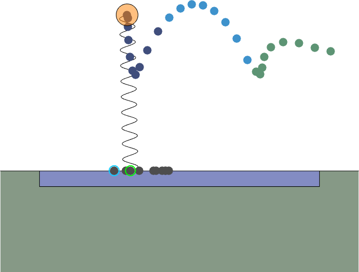
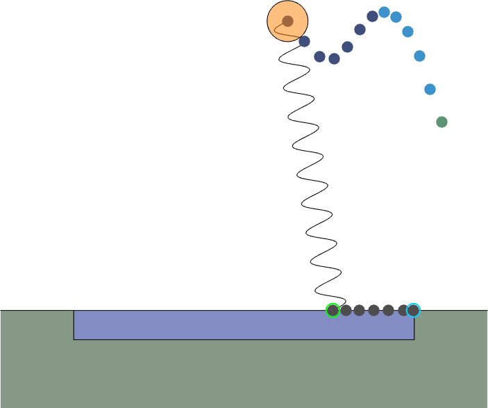
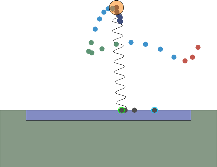
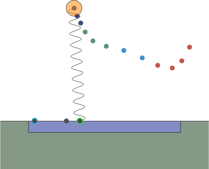
Visualization of trajectories and other stuff relevant to my research project (more on that later) is on GitHub. Include visualize.m, animate.m, VisParams.m, and rewind.gif to look at the optimized trajectories. My apologies for the slightly messy code. Here’s some images of what the trajectories look like:

Key: dark blue (slide phase), green (first stick phase), red (second stick phase), light blue (flight phase), black (toe position), green highlight (landing), blue highlight (takeoff)—dots equally time-spaced, SLIP in starting state.